Sort according to the data you want to outline. … Select the Data tab, then locate the Outline group.Click the Subtotal command to open the Subtotal dialog box. … In the At each change in field, select the column you want to use to outline your worksheet.
How do you collapse the whole outline to show only the subtotals in Excel?
To collapse a group of cells, click a minus sign. You can use the numbers to collapse or expand groups by level. For example, click the 2 to only show the subtotals.
How do you outline data in Excel?
- Select a cell in the range of cells you want to outline.
- On the Data tab, in the Outline group, click the arrow under Group, and then click Auto Outline.
How do you use the outline symbols to display only the subtotal rows?
2. In the Excel Options dialog box, click Advanced, and go to Display options for this worksheet section, specify the worksheet that you want to show or hide the outline symbols from the drop down list, then check or uncheck Show outline symbols if an outline is applied as you need to show or hide the outline symbols.How do you collapse an outline to show subtotals?
Go to the Data menu in the ribbon and look in the Outline group. Click on the Subtotal command. Select how you want it subtotaled (in our example, this would be by location and for each of the ice cream treat categories). Click OK.
How do you use Subtotal outlines?
- Sort according to the data you want to outline. …
- Select the Data tab, then locate the Outline group.
- Click the Subtotal command to open the Subtotal dialog box. …
- In the At each change in field, select the column you want to use to outline your worksheet.
How do you Uncollapse rows Excel?
- To unhide all hidden rows in Excel, navigate to the “Home” tab.
- Click “Format,” which is located towards the right hand side of the toolbar.
- Navigate to the “Visibility” section. …
- Hover over “Hide & Unhide.”
- Select “Unhide Rows” from the list.
Why Excel Cannot create an outline?
It’s in the Group drop-down menu. If you receive a pop-up box that says “Cannot create an outline”, your data doesn’t have an outline-compatible formula in it. You’ll need to manually outline the data.How do you create an outline in a table in Excel?
- Select a cell or a range of cells to which you want to add borders.
- On the Home tab, in the Font group, click the down arrow next to the Borders button, and you will see a list of the most popular border types.
- Click the border you want to apply, and it will be immediately added to the selected cells.
To add collapsible Excel rows, simply select the rows you want to collapse and use the Outline feature under the Data tab to group them. You can then click the plus and minus symbols on the left to collapse and expand, or the numbers at the top to collapse all and expand all.
Article first time published onWhy would you click the collapse outline symbol above a column of outlined data?
Why would you click the collapse outline symbol above a column of outlined data? You want to hide the detailed columns to focus on the result column.
How do you outline cells in Excel 2016?
- Right-click and then select “Format Cells” from the popup menu.
- When the Format Cells window appears, select the Border tab. Next select your line style and the borders that you wish to draw. …
- Now when you return to your spreadsheet, you should see the border, as follows:
- NEXT.
How do I make Excel cells expand to fit text?
Select the row or rows that you want to change. On the Home tab, in the Cells group, click Format. Under Cell Size, click AutoFit Row Height. Tip: To quickly autofit all rows on the worksheet, click the Select All button, and then double-click the boundary below one of the row headings.
How do you freeze the top row of a worksheet?
- Scroll your spreadsheet until the row you want to lock in place is the first row visible under the row of letters.
- In the menu, click “View.”
- In the ribbon, click “Freeze Panes” and then click “Freeze Top Row.”
How do I make a thick outside border in Excel?
Select one or more cells that have a border that you want to change. Right-click over the cells you’ve chosen and select Format Cells and, in the popup window, click the Border tab. For a continuous line, choose one of the thicker styles from the Line box. In the Presets section, click your existing border type.
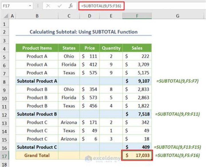
How Subtotal function works in Excel?
Use the SUBTOTAL function to exclude filtered or hidden rows when calculating a total. You can choose any one of the 11 functions that SUBTOTAL can calculate, such as Sum, Average, Count or Max. This video show how to use SUBTOTAL or the newer AGGREGATE function, to work with filtered data.
How do I use grouping in Excel?
- Select the rows or columns you want to group. In this example, we’ll select columns B, C, and D.
- Select the Data tab on the Ribbon, then click the Group command.
- The selected rows or columns will be grouped. In our example, columns B, C, and D are grouped.
How do you outline text in Excel?
If you are using Excel or PowerPoint To add the same outline to text in multiple places, select the first piece of text, and then press and hold CTRL while you select the other pieces of text. To add or change an outline color, click the color that you want. To choose no color, click No Outline.
What does Vlookup mean in Excel?
VLOOKUP stands for ‘Vertical Lookup‘. It is a function that makes Excel search for a certain value in a column (the so called ‘table array’), in order to return a value from a different column in the same row.
How do I set up automatic subtotals?
- On the Data tab, in the Outline group, click Subtotal. The Subtotal dialog box is displayed.
- In the At each change in box, click the nested subtotal column. …
- In the Use function box, click the summary function that you want to use to calculate the subtotals. …
- Clear the Replace current subtotals check box.
How do you automatically hide columns in Excel?
- How to group columns. Select all columns you want to group and go to the menu Data >> Group. That’s all J The hide button will be displayed next to the last column above.
- How to group rows. It’s the same as columns. …
- Automatic group columns and rows. Excel can create all groups in one step.
What is the shortcut for grouping in Excel?
The shortcut for grouping rows or columns in Excel is Alt Shift right arrow in Windows and Command Shift K on a Mac. If you only have cells selected (not entire rows or columns) this shortcut will cause Excel to display the Group dialog box. There, you can tell Excel to group either Rows or Columns.
How do I put a border around a cell in Excel?
Select the cells you want to format. Click the down arrow beside the Borders button in the Font group on the Home tab. A drop-down menu appears, with all the border options you can apply to the cell selection. Use the Borders button on the Home tab to choose borders for the selected cells.
How do you group rows on excel and expand and collapse?
First, select the rows that need to be grouped. Now press the shortcut key SHIFT + ALT + Right Arrow Key to group these rows. In the above, we have seen how to group the data and how to group row with expand and collapse option by using PLUS & MINUS icons.
How do you group multiple rows in Excel?
- Select the rows or columns you want to group. In this example, we’ll select columns A, B, and C. …
- Select the Data tab on the Ribbon, then click the Group command. Clicking the Group command.
- The selected rows or columns will be grouped. In our example, columns A, B, and C are grouped together.